In the first part of this post I present an update on the profitability for Light Tight Oil (LTO) extraction in the Bakken (ND) as one big project.
This is followed with economic life cycle analysis for the average LTO well of the 2014, 2015 and 2016 vintages in the Bakken.
This analysis found that companies in aggregate continue to outspend net cash flows from operations and for 2017 this is now expected to total $2 – $3 Billion.
- The strong growth and sustained high LTO extraction from the Bakken were facilitated by considerable amounts of debts. The growth in total debts outstanding (employed capital) continues to grow, albeit at a slower pace.
- With oil prices sustained at present levels the total employed capital (primarily debt) constitutes severe obstacles for the profitability for the Bakken.
- In a scenario where no wells were added post 2017 and the wellhead (at WH) price remained at $40/bo [~ $50/bo WTI] estimated losses for the project would be $20 – $22 Billion.
- In a scenario where no wells were added post 2017 and the wellhead price remained at $60/bo [~ $70/bo WTI], the payout was reached after 7,5 years (in 2025) and the estimated return for the project becomes 3,5%.
- With a sustained wellhead price at $74/bo [~ $84/bo WTI] post 2017, the payout was reached after 4,3 years (in 2022) and the estimated return becomes 7%.
What makes the profitability for the Bakken challenging are the number of years front loaded with negative cash flows. - So far the recent years improvements in flow and Estimated Ultimate Recovery (EUR) have not entirely caught up with the decline in and the sustained lower oil price.
- For the average 2016 vintage well it was estimated that a sustained oil price of $53/bo at WH [~ $63/bo WTI] would return 7%.

Figure 01: The chart above shows the estimated rolling 12 months totals [black columns] net cash flows. The red area shows the estimated cumulative net cash flow since Jan-09 and per Jul-17. LOE, G&A and interest rates (effective, i.e. adjusted for tax effects) based on a weighted average from several companies’ SEC 10-K/Q filings. Taxes according to what has been in force. Price of oil, North Dakota Sweet (NDS) and realized gas price as reported by several companies.

In the Bakken(ND) and since January 2009 and per July 2017 an estimated $100 Billion has been used for manufacturing operational LTO wells and at end July 2017 an estimated $35 Billion were outstanding to be recovered from the estimated remaining proven developed producing (PDP) reserves.
At the most CAPEX for well manufacturing in the Bakken out spent cash flow from operations at an annual rate of $9 Billion. For the Bakken there has been two distinct CAPEX cycles, the first in 2011/2012 while the oil price remained high, followed by another in 2015 after the collapse in the oil price.
The second cycle may have been rationalized by several factors like an expected rebound in the oil price, which OPEC (primarily its Middle East members) helped derail through their rapid increase in oil supplies starting in early 2015 in an (believed) effort to fight for market share. The second cycle may also have been rationalized by the incentive structure for management of LTO companies in which these were rewarded by volume growth over profitability.
Incurred costs for drilled, uncompleted wells (DUCs) and salt water disposal wells (SWDs) are not included. Directors cut for September 2017 listed 889 wells waiting for completion. Costs from any heavy and costly well maintenance/interventions are not included.
The DUCs represents $2,2 – $2,7 Billion in capital employed.
For the Bakken as one big project and the life cycle analysis the gross interest costs of 6% were reduced by 35% to reflect corporate tax effects.
Effects from hedges and from bankruptcy proceedings (debt restructuring) are not included.
Any arbitrage from the realized oil price adjusted for wellhead price, transport costs and any tax effects from this arbitrage are not included.
Some companies are now recirculating primarily borrowed money (at some interest) from the net operating cash flow and injecting additional capital to continue the manufacturing of new wells.

Specific interest cost is not adjusted for legacy flow prior to 2009.
Life cycle analysis
One good way to understand the profitability of shale oil wells is to establish each well as a profit/loss center.
This helps quantify specific LOE, G&A and interest cost/expenses as the well depletes and shows the recovery of capital employed on its way towards payout and profits generated.
Look at it this way, manufacturing a well at $7M – $9M is like borrowing that well what it costs with an interest of 6% (used here) pa and the principal (investment in the well) is paid down with the surplus post taxes, OPEX (inclusive G&A) and interest expenses.
Here some readers may object as a small portion of the well costs may be equity and the rest is debt.
The challenge here is to split out the portions of the well’s investments that are equity and debt.
Any investor would evaluate alternative returns for equity and using the equity for manufacturing a well ought (at least) to have the same return as (real, tax adjusted) interests on debt (cost of borrowed capital). As long equity is employed it should at least return the same as the costs of the debt. Companies with a good credit rating (low costs of borrowing) have some edge here.
If (employed) equity comes with no return requirement, it would, over time, gradually lose value due to inflation.
This is something that does not show up in most companies’ financial statements. Individual companies may have different requirements for return on equity and different practices for treatment of equity.
The chart below shows how recovery of employed capital (investment) develops for an average well in the Bakken for the 2014, 2015 and 2016 vintages started in January.

More about the assumptions used at the end of this article.
Refer also figure 09 showing projected trajectories for gross specific interest costs with $40/bo at WH.
The average well represents the arithmetic average for all the wells of some specific vintage or month. The economics of the average well describes the economics for that specific population of wells. If the average well shows a positive return, it means the whole population of wells comes out with a profit, even if there are wide differences in profitability amongst the individual wells. Some (individual) wells can be very profitable while the poorest incurs various degrees of losses (that have to be carried by the better wells).
Therefore there will also be differences amongst companies depending on the quality [productivity] of their well population (also referred to as acreage held).

More about the assumptions used at the end of this article.
As figure 04 shows a higher oil price allows for a more rapid recovery of the employed capital (investment) and a lowered trajectory for specific interest costs, ref also figure 10. And vice versa.

Well economics are very much dependent on how its (improved) flow hits the oil price as shown in figures 03, 04 and 05.
With sustained low oil prices the economics of LTO wells becomes very sensitive to the realized oil price during its first 2 – 3 years of flow and less sensitive to improvements in productivity.
For the average 2016 vintage well it was estimated that a sustained oil price of $53/bo at WH [~ $63/bo WTI] would return 7%.
For the average 2016 well an increase in the royalty from 18% to 20% would increase the price to reach payout by $1/bo and about $1,50/bo for a 7% return.
So far actual oil prices have been lower. The effects from this is that it requires a higher oil price for the remaining estimated recoverable oil (and gas) to reach payout and some specified return.
For the 2016 average well started in Jan-16 it was estimated that payout would be reached with a sustained price of $60/bo at WH [~ $70/bo WTI] and a 7% return with $78/bo at WH [~ $88/bo WTI] as from Oct-17.
For a well started in Dec-16, the payout would be reached with a sustained $50/bo at WH [~ $60/bo WTI] and 7% return with $65/bo at WH [~ $75/bo WTI] as from Oct-17.
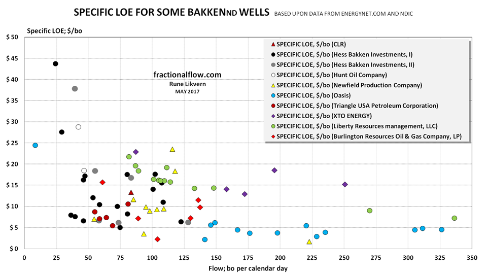
Presently there are limited available data on frequencies and financial costs on late life heavy well interventions. Therefore, some duly caution should be applied to the data in figure 06 though it should be expected that the general direction with higher specific LOE as the well ages and the flow declines is valid.
Any shut ins requiring heavy well interventions should be expected to constitute a set back for the profitability due to deferred recovery of remaining outstanding employed capital and additional costs.
Figure 06 is based on Joint Interest Billings (JIB) covering periods of mostly 6 months for 81 wells started as from Jun-10 to Jul- 16. These JIBs covered various activities like casing repair jobs, heavy work overs requiring considerable rig time and equipment charges.
Royalties for the wells in figure 06 varied from 17% to 25%.
The work presented in figure 06 was carried out last winter/spring with a colleague/friend (lawyer educated) in the US oil industry and represents data on 81 wells (of which 2 are off the chart).
The data were mined from EnergyNet which is an oil and gas marketplace.
Assumptions
Unless otherwise stated the oil price [at the wellhead; at WH] used is for North Dakota Sweet (NDS), from Flint Hills. The spread used between WTI and NDS is $10/bo. Since January 2014 this spread has averaged close to $13/bo.
Unless otherwise specified, royalties of 18% have been used in this article.
Most royalties were found to be in the span of 17% to 25%. The lower the royalty the lower the required price to reach payout and some specific return becomes.
Developments in General & Administration (G&A) were derived from several companies SEC 10-K/Q filings and this was now found to be about $5/bo.

Figure 07 shows that with time there have been noticeable flow and EUR improvements (productivities) for the wells during their first 2-3 years of operation. If this holds up will be known some time in the future by comparing the cumulative from different vintages over 8 – 10 years of flow.
To avoid confusion in this post by using Barrels of Oil Equivalents (BOE), which is appropriate for energy accounting, all costs in this post are carried by the oil then the realized sale price for natural gas/NGLs, post tax and royalty adjustments, was added to the net back from oil. Gas volumes derived from the development in the Gas to Oil Ratio (GOR).
Converting natural gas to BOE results in higher reported volumes which lowers the specific costs [$/BOE]. Sale price realized for one BOE of natural gas has been 25% – 50% of that of one barrel of LTO.
From several companies, that is primarily exposed to the Bakken, it was derived from their SEC 10-Q/K filings and their reporting with BOE and by moving in and out of BOE and Mcf, that these had lost on average $1 – $2/Mcf since 2015.
GOR for the Bakken is now at about 1,8 Mcf/bo.
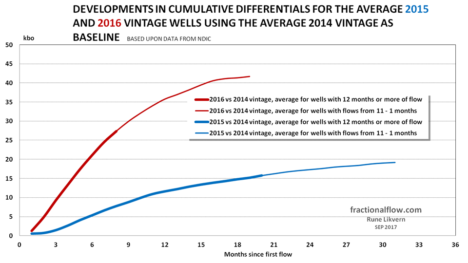
So far and over time there has been noticeable improvements in the well productivities expressed as cumulative LTO over time for the most recent wells. This is primarily due to longer laterals and improved use of the number of fracking stages and proppants.
In this context, it would be interesting to use a supplemental metric like developments in specific LTO productivity per unit length of lateral, like bo/d/100 ft.
The average 2017 vintage of wells has (so far) higher cumulatives and the higher oil price places these on a more favorable trajectory towards payout than the 2016 vintage, and the future oil price will become decisive for reaching payout and producing profits.
In this analysis an effective interest for debts and equity of 6% has been applied. The interest was found to vary amongst companies in the Bakken depending on their credit rating (assets and equity) and was below 4% of some majors and above 8% for small independents. A weighted interest of 6% was derived from several companies’ SEC 10 K/Q filings, that had their primary exposure to the Bakken.
As of now constraint was applied about speculating on how interest rates would develop in the future for LTO companies as these may roll over some of their debts some years into the future. Variables here are the central banks’ policies and developments in companies’ assets/equity and credit ratings.
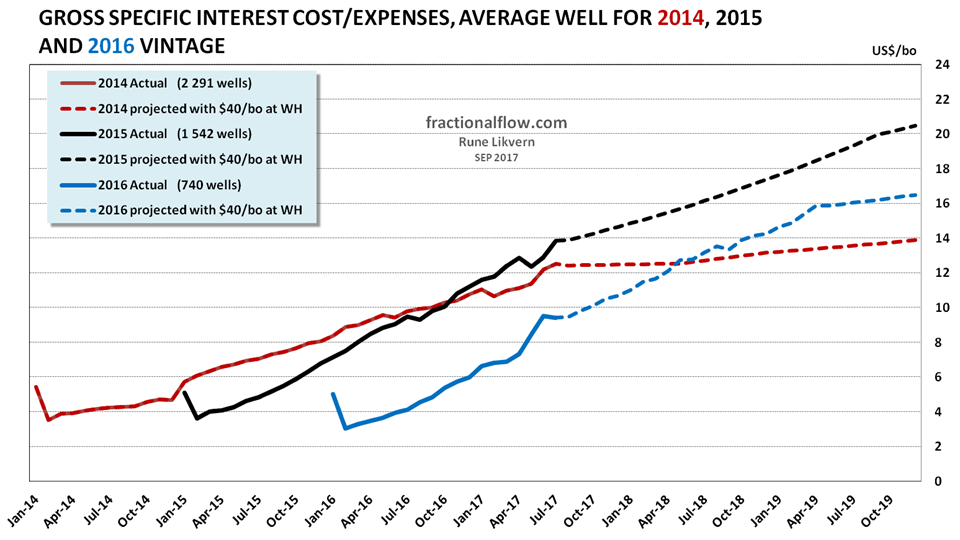
Effective interest of 6% used on outstanding debts (and equity).
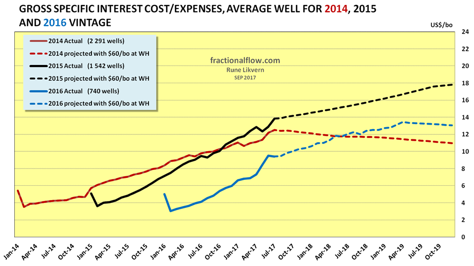
Effective interest of 6% used on outstanding debts (and equity).
What figure 09 and 10 illustrates is that the higher the oil price is, the faster the recovery of employed capital becomes which leads to a lowered trajectory for the specific interest expenses.
Interest costs as from payment of the first invoice from manufacturing a well was estimated somewhere between $100k – $150k and assumed included in the well costs.
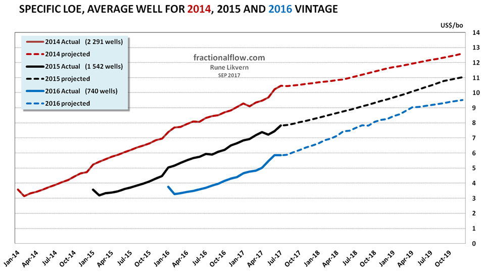
Lease and Operating Expenses (LOE) are defined by a fixed monthly amount plus an amount related to growing gas and water production (treatment and disposal) and has its low at $3/bo (as the flow is highest) and grows with declining oil production, growth in GOR and water cut, refer also figure 06.
Data on the wells in the Bakken has kindly been provided by Enno Peters at shaleprofile.com.
Readers are encouraged to visit Enno’s excellent site to study and customize visualizations of tons of actual data from all major US shale plays that are updated monthly.

You must be logged in to post a comment.